Data Analytics for Business: Excel’ Tips for Beginner

Dynamic Calculation & Logical Case IF, Dynamic Lookup

The dataset that I used for training is Supermarket Sales.

Dynamic Calculation & Logical Case IF

Tips 1. Quickly block columns/rows in a table automatically

If CTRL + A will block the entire table, then this tip will help if you only need specific columns or rows.

Windows: CTRL + Shift + Arrow Button

Macbook: CMD + Shift + Arrow Button

Tips 2. Create dynamic table

Automatic tables will be useful when you have written a formula in a certain column/row range and one day you will add data to the table. So, there is no need to change the data range in the formula.

1. CTRL + A on table areas that are not yet dynamic tables
2. CTRL + T
3. Click OK

Tables that have become automatic, will change with the following characteristics.

The data range formula becomes the title of the dynamic table, for example the original =AVERAGE(H3:H22) becomes =AVERAGE(Table[ColumnName])

Tips 3. If there is more than 1 logical test, it is necessary to use the LOGICAL OPERATOR

Logical Operators are divided into 2, namely OR (one of them) and AND (all of them are required)

Case: If the total sales (Total) is more than 100k and the total items (Quantity) is more than 3, then it reaches the target.

Using the IF formula and utilizing the logical AND operator and the TRUE value is “Mencapai Target (Achieved Target)” so that each row will display a description of each sale.

=IF(AND(Table[Total] > 100000; Table[Quantity] > 3); “Mencapai Target” ; “Tidak Mencapai Target”)

It is different if the case becomes “…the total sales (Total) is more than 100k or the total goods (Quantity) is more than 3..”

Then use the IF formula and utilize the logical OR operator

=IF(OR(Table[Total] > 100000; Table[Quantity] > 3); “Mencapai Target” ; “Tidak Mencapai Target”)

Dynamic Lookup

Pivot tables make it possible to summarize, analyze, and display data in an interactive table format, so we can easily find trends, patterns, and comparisons in the data quickly.

Tips 1. Convert dynamic table into pivot table

1. CTRL + A in the table area
2. Menu > Insert > Pivot Table
3. Click OK

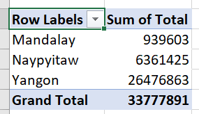
For example, I want to see the total sales by city.

In a matter of seconds, the comparison immediately appears without using a formula.

Tips 2. Filtering pivot table with slicer

Why slicer? Because the data analysis display will be more convenient and easy to read.

1. Click the table area
2. Menu > Insert > Slicer
3. Select which category you want (to see the total sales)

For example, viewing total sales by product type. Then choose product line.

The slicer result display will look like this:

More eye-catching, right?

What other tips do you think would be useful in data analytics for business?